how to prove a hypothesis wrong

• Translation

Responding to a Disproven or Failed Research Hypothesis

By charlesworth author services.

• Charlesworth Author Services
• 03 August, 2022

When meeting with a disproven or failed hypothesis , after having expended so much time and effort, precisely how should researchers respond? Responding well to a disproven or failed hypothesis is an essential component to scientific research . As a researcher, it helps to learn ‘ research resilience ’: the ability to carefully analyse, effectively document and broadly disseminate the failed hypotheses, all with an eye towards learning and future progress. This article explores common reasons why a hypothesis fails, as well as specific ways you can respond and lessons you can learn from this. 

Note : This article assumes that you are working on a hypothesis (not a null hypothesis): in other words, you are seeking to prove that the hypothesis is true, rather than to disprove it. 

Reasons why a hypothesis is disproven/fails

Hypotheses are disproved or fail for a number of reasons, including:

• The researcher’s preconception is incorrect , which leads to a flawed and failed hypothesis.
• The researcher’s findings are correct, but those findings aren’t relevant .
• Data set/sample size may not be sufficiently large to yield meaningful results. (If interested, learn more about this here: The importance of having Large Sample Sizes for your research )
• The hypothesis itself lies outside the realm of science . The hypothesis cannot be tested by experiments for which results have the potential to show that the idea is false.

Responding to a disproved hypothesis

After weeks or even months of intense thinking and experimenting, you have come to the conclusion that your hypothesis is disproven. So, what can you do to respond to such a disheartening realisation? Here are some practical steps you can take.

• Analyse the hypothesis carefully, as well as your research.   Performing a rigorous, methodical ‘post-mortem’ evaluation of your hypothesis and experiments will enable you to learn from them and to effectively and efficiently share your reflections with others. Use the following questions to evaluate how the research was conducted: 
• Did you conduct the experiment(s) correctly? 
• Was the study sufficiently powered to truly provide a definitive answer?
• Would a larger, better powered study – possibly conducted collaboratively with other research centres – be necessary, appropriate or helpful? 
• Would altering the experiment — or conducting different experiments — more appropriately answer your hypothesis? 
• Share the disproven hypothesis, and your experiments and analysis, with colleagues. Sharing negative data can help to interpret positive results from related studies and can aid you to adjust your experimental design .
• Consider the possibility that the hypothesis was not an attempt at gaining true scientific understanding, but rather, was a measure of a prevailing bias .

Positive lessons to be gained from a disproved hypothesis

Even the most successful, creative and thoughtful researchers encounter failed hypotheses. What makes them stand out is their ability to learn from failure. The following considerations may assist you to learn and gain from failed hypotheses:

• Failure can be beneficial if it leads directly toward future exploration.
• Does the failed hypothesis definitively close the door on further research? If so, such definitive knowledge is progress.
• Does the failed hypothesis simply point to the need to wait for a future date when more refined experiments or analysis can be conducted? That knowledge, too, is useful. 
• ‘Atomising’ (breaking down and dissecting) the reasoning behind the conceptual foundation of the failed hypothesis may uncover flawed yet correctable thinking in how the hypothesis was developed. 
• Failure leads to investigation and creativity in the pursuit of viable alternative hypotheses, experiments and statistical analyses. Better theoretical or experimental models often arise out of the ashes of a failed hypothesis, as do studies with more rigorously attained evidence (such as larger-scale, low-bias meta-analyses ). 

Considering a post-hoc analysis

A failed hypothesis can then prompt you to conduct a post-hoc analysis. (If interested, learn more about it here: Significance and use of Post-hoc Analysis studies )

All is not lost if you conclude you have a failed hypothesis. Remember: A hypothesis can’t be right unless it can be proven wrong.  Developing research resilience will reward you with long-term success.

Maximise your publication success with Charlesworth Author Services.

Charlesworth Author Services, a trusted brand supporting the world’s leading academic publishers, institutions and authors since 1928.

To know more about our services, visit: Our Services

Share with your colleagues

Scientific Editing Services

Sign up – stay updated.

We use cookies to offer you a personalized experience. By continuing to use this website, you consent to the use of cookies in accordance with our Cookie Policy.

Back to Blog home

Hypothesis testing explained in 4 parts, yuzheng sun, phd.

As data scientists, Hypothesis Testing is expected to be well understood, but often not in reality. It is mainly because our textbooks blend two schools of thought – p-value and significance testing vs. hypothesis testing – inconsistently.

For example, some questions are not obvious unless you have thought through them before:

Are power or beta dependent on the null hypothesis?

Can we accept the null hypothesis? Why?

How does MDE change with alpha holding beta constant?

Why do we use standard error in Hypothesis Testing but not the standard deviation?

Why can’t we be specific about the alternative hypothesis so we can properly model it?

Why is the fundamental tradeoff of the Hypothesis Testing about mistake vs. discovery, not about alpha vs. beta?

Addressing this problem is not easy. The topic of Hypothesis Testing is convoluted. In this article, there are 10 concepts that we will introduce incrementally, aid you with visualizations, and include intuitive explanations. After this article, you will have clear answers to the questions above that you truly understand on a first-principle level and explain these concepts well to your stakeholders.

We break this article into four parts.

Set up the question properly using core statistical concepts, and connect them to Hypothesis Testing, while striking a balance between technically correct and simplicity. Specifically, 

We emphasize a clear distinction between the standard deviation and the standard error, and why the latter is used in Hypothesis Testing

We explain fully when can you “accept” a hypothesis, when shall you say “failing to reject” instead of “accept”, and why

Introduce alpha, type I error, and the critical value with the null hypothesis

Introduce beta, type II error, and power with the alternative hypothesis

Introduce minimum detectable effects and the relationship between the factors with power calculations , with a high-level summary and practical recommendations

Part 1 - Hypothesis Testing, the central limit theorem, population, sample, standard deviation, and standard error

In Hypothesis Testing, we begin with a null hypothesis , which generally asserts that there is no effect between our treatment and control groups. Commonly, this is expressed as the difference in means between the treatment and control groups being zero.

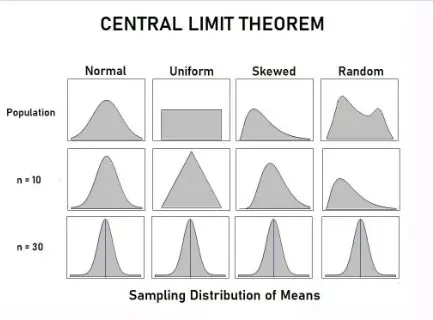
The central limit theorem suggests an important property of this difference in means — given a sufficiently large sample size, the underlying distribution of this difference in means will approximate a normal distribution, regardless of the population's original distribution. There are two notes:

1. The distribution of the population for the treatment and control groups can vary, but the observed means (when you observe many samples and calculate many means) are always normally distributed with a large enough sample. Below is a chart, where the n=10 and n=30 correspond to the underlying distribution of the sample means.

2. Pay attention to “the underlying distribution”. Standard deviation vs. standard error is a potentially confusing concept. Let’s clarify.

Standard deviation vs. Standard error

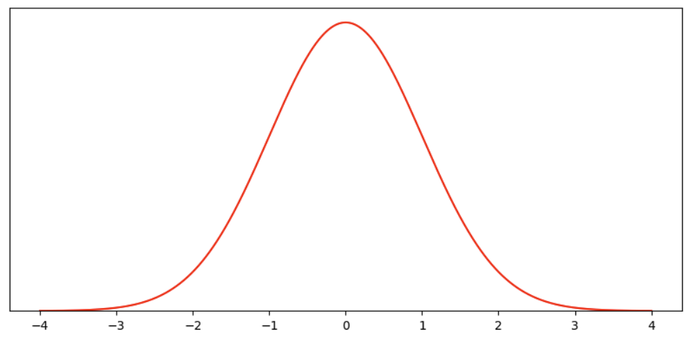
Let’s declare our null hypothesis as having no treatment effect. Then, to simplify, let’s propose the following normal distribution with a mean of 0 and a standard deviation of 1 as the range of possible outcomes with probabilities associated with this null hypothesis.

The language around population, sample, group, and estimators can get confusing. Again, to simplify, let’s forget that the null hypothesis is about the mean estimator, and declare that we can either observe the mean hypothesis once or many times. When we observe it many times, it forms a sample*, and our goal is to make decisions based on this sample.

* For technical folks, the observation is actually about a single sample, many samples are a group, and the difference in groups is the distribution we are talking about as the mean hypothesis. The red curve represents the distribution of the estimator of this difference, and then we can have another sample consisting of many observations of this estimator. In my simplified language, the red curve is the distribution of the estimator, and the blue curve with sample size is the repeated observations of it. If you have a better way to express these concepts without causing confusiongs, please suggest.

This probability density function means if there is one realization from this distribution, the realitization can be anywhere on the x-axis, with the relative likelihood on the y-axis.

If we draw multiple observations , they form a sample . Each observation in this sample follows the property of this underlying distribution – more likely to be close to 0, and equally likely to be on either side, which makes the odds of positive and negative cancel each other out, so the mean of this sample is even more centered around 0.

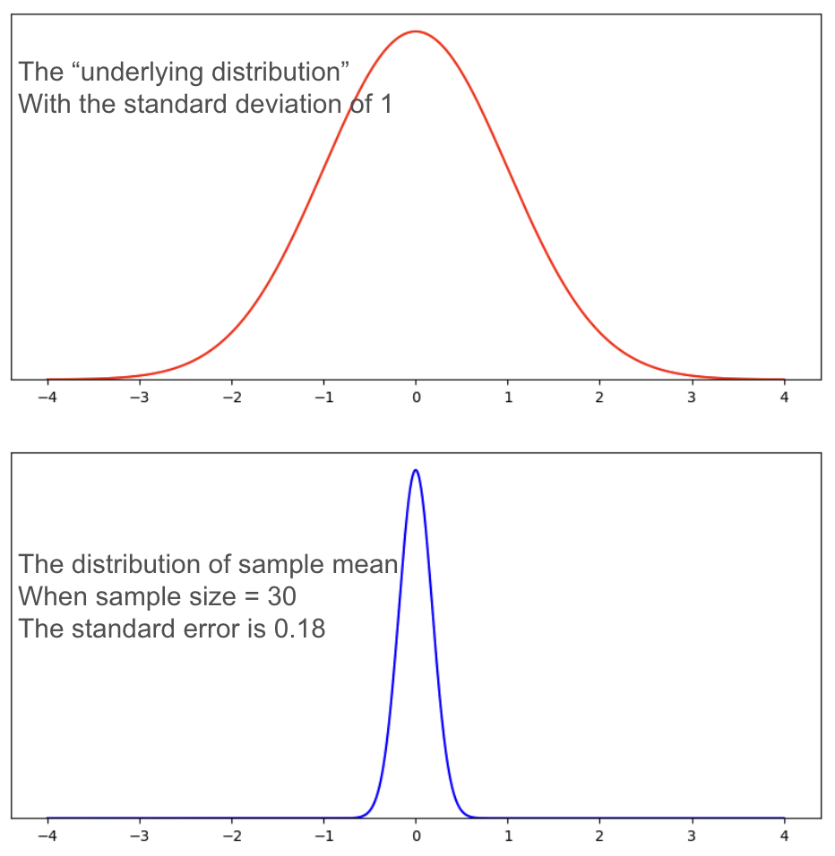
We use the standard error to represent the error of our “sample mean” . 

The standard error = the standard deviation of the observed sample / sqrt (sample size). 

For a sample size of 30, the standard error is roughly 0.18. Compared with the underlying distribution, the distribution of the sample mean is much narrower.

In Hypothesis Testing, we try to draw some conclusions – is there a treatment effect or not? – based on a sample. So when we talk about alpha and beta, which are the probabilities of type I and type II errors , we are talking about the probabilities based on the plot of sample means and standard error .

Part 2, The null hypothesis: alpha and the critical value

From Part 1, we stated that a null hypothesis is commonly expressed as the difference in means between the treatment and control groups being zero.

Without loss of generality*, let’s assume the underlying distribution of our null hypothesis is mean 0 and standard deviation 1

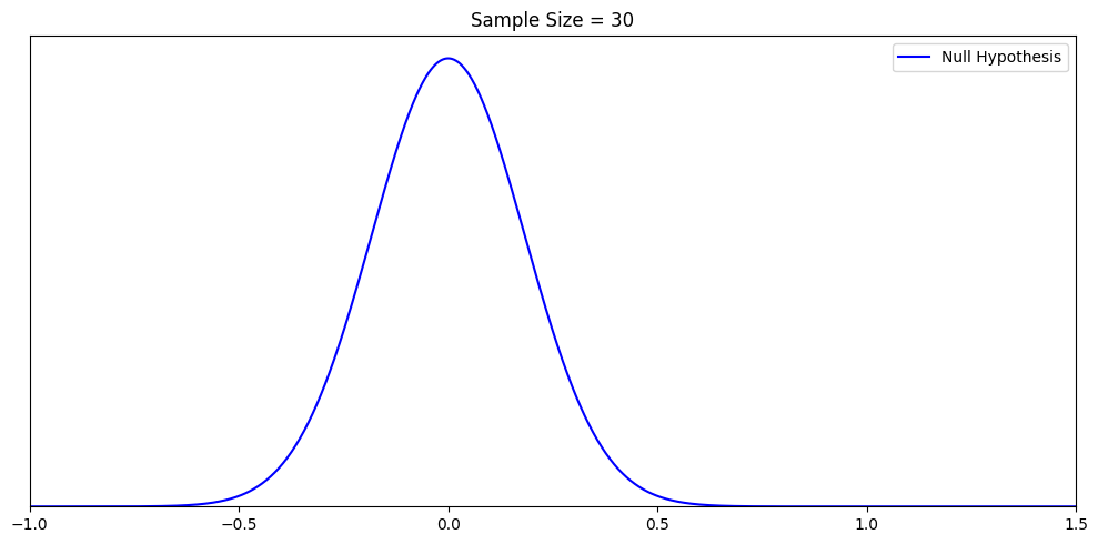
Then the sample mean of the null hypothesis is 0 and the standard error of 1/√ n, where n is the sample size.

When the sample size is 30, this distribution has a standard error of ≈0.18 looks like the below. 

*: A note for the technical readers: The null hypothesis is about the difference in means, but here, without complicating things, we made the subtle change to just draw the distribution of this “estimator of this difference in means”. Everything below speaks to this “estimator”.

The reason we have the null hypothesis is that we want to make judgments, particularly whether a  treatment effect exists. But in the world of probabilities, any observation, and any sample mean can happen, with different probabilities. So we need a decision rule to help us quantify our risk of making mistakes.

The decision rule is, let’s set a threshold. When the sample mean is above the threshold, we reject the null hypothesis; when the sample mean is below the threshold, we accept the null hypothesis.

Accepting a hypothesis vs. failing to reject a hypothesis

It’s worth noting that you may have heard of “we never accept a hypothesis, we just fail to reject a hypothesis” and be subconsciously confused by it. The deep reason is that modern textbooks do an inconsistent blend of Fisher’s significance testing and Neyman-Pearson’s Hypothesis Testing definitions and ignore important caveats ( ref ). To clarify:

First of all, we can never “prove” a particular hypothesis given any observations, because there are infinitely many true hypotheses (with different probabilities) given an observation. We will visualize it in Part 3.

Second, “accepting” a hypothesis does not mean that you believe in it, but only that you act as if it were true. So technically, there is no problem with “accepting” a hypothesis.

But, third, when we talk about p-values and confidence intervals, “accepting” the null hypothesis is at best confusing. The reason is that “the p-value above the threshold” just means we failed to reject the null hypothesis. In the strict Fisher’s p-value framework, there is no alternative hypothesis. While we have a clear criterion for rejecting the null hypothesis (p < alpha), we don't have a similar clear-cut criterion for "accepting" the null hypothesis based on beta.

So the dangers in calling “accepting a hypothesis” in the p-value setting are:

Many people misinterpret “accepting” the null hypothesis as “proving” the null hypothesis, which is wrong; 

“Accepting the null hypothesis” is not rigorously defined, and doesn’t speak to the purpose of the test, which is about whether or not we reject the null hypothesis. 

In this article, we will stay consistent within the Neyman-Pearson framework , where “accepting” a hypothesis is legal and necessary. Otherwise, we cannot draw any distributions without acting as if some hypothesis was true.

You don’t need to know the name Neyman-Pearson to understand anything, but pay attention to our language, as we choose our words very carefully to avoid mistakes and confusion.

So far, we have constructed a simple world of one hypothesis as the only truth, and a decision rule with two potential outcomes – one of the outcomes is “reject the null hypothesis when it is true” and the other outcome is “accept the null hypothesis when it is true”. The likelihoods of both outcomes come from the distribution where the null hypothesis is true.

Later, when we introduce the alternative hypothesis and MDE, we will gradually walk into the world of infinitely many alternative hypotheses and visualize why we cannot “prove” a hypothesis.

We save the distinction between the p-value/significance framework vs. Hypothesis Testing in another article where you will have the full picture.

Type I error, alpha, and the critical value

We’re able to construct a distribution of the sample mean for this null hypothesis using the standard error. Since we only have the null hypothesis as the truth of our universe, we can only make one type of mistake – falsely rejecting the null hypothesis when it is true. This is the type I error , and the probability is called alpha . Suppose we want alpha to be 5%. We can calculate the threshold required to make it happen. This threshold is called the critical value . Below is the chart we further constructed with our sample of 30.

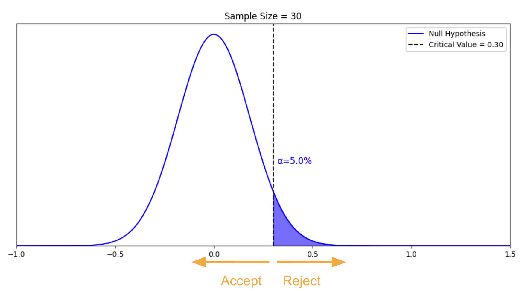
In this chart, alpha is the blue area under the curve. The critical value is 0.3. If our sample mean is above 0.3, we reject the null hypothesis. We have a 5% chance of making the type I error.

Type I error: Falsely rejecting the null hypothesis when the null hypothesis is true

Alpha: The probability of making a Type I error

Critical value: The threshold to determine whether the null hypothesis is to be rejected or not

Part 3, The alternative hypothesis: beta and power

You may have noticed in part 2 that we only spoke to Type I error – rejecting the null hypothesis when it is true. What about the Type II error – falsely accepting the null hypothesis when it is not true?

But it is weird to call “accepting” false unless we know the truth. So we need an alternative hypothesis which serves as the alternative truth. 

Alternative hypotheses are theoretical constructs

There is an important concept that most textbooks fail to emphasize – that is, you can have infinitely many alternative hypotheses for a given null hypothesis, we just choose one. None of them are more special or “real” than the others. 

Let’s visualize it with an example. Suppose we observed a sample mean of 0.51, what is the true alternative hypothesis?

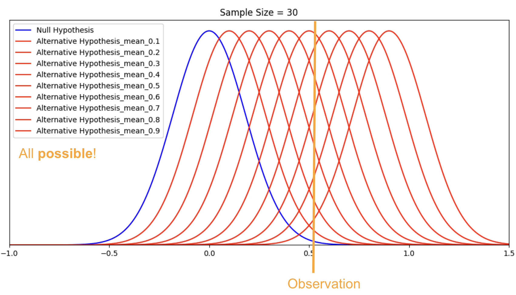
With this visualization, you can see why we have “infinitely many alternative hypotheses” because, given the observation, there is an infinite number of alternative hypotheses (plus the null hypothesis) that can be true, each with different probabilities. Some are more likely than others, but all are possible.

Remember, alternative hypotheses are a theoretical construct. We choose one particular alternative hypothesis to calculate certain probabilities. By now, we should have more understanding of why we cannot “accept” the null hypothesis given an observation. We can’t prove that the null hypothesis is true, we just fail to accept it given the observation and our pre-determined decision rule. 

We will fully reconcile this idea of picking one alternative hypothesis out of the world of infinite possibilities when we talk about MDE. The idea of “accept” vs. “fail to reject” is deeper, and we won’t cover it fully in this article. We will do so when we have an article about the p-value and the confidence interval.

Type II error and Beta

For the sake of simplicity and easy comparison, let’s choose an alternative hypothesis with a mean of 0.5, and a standard deviation of

1. Again, with a sample size of 30, the standard error ≈0.18. There are now two potential “truths” in our simple universe.

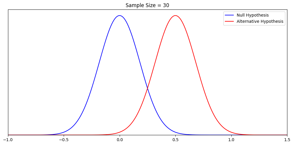
Remember from the null hypothesis, we want alpha to be 5% so the corresponding critical value is 0.30. We modify our rule as follows:

If the observation is above 0.30, we reject the null hypothesis and accept the alternative hypothesis ; 

If the observation is below 0.30, we accept the null hypothesis and reject the alternative hypothesis .

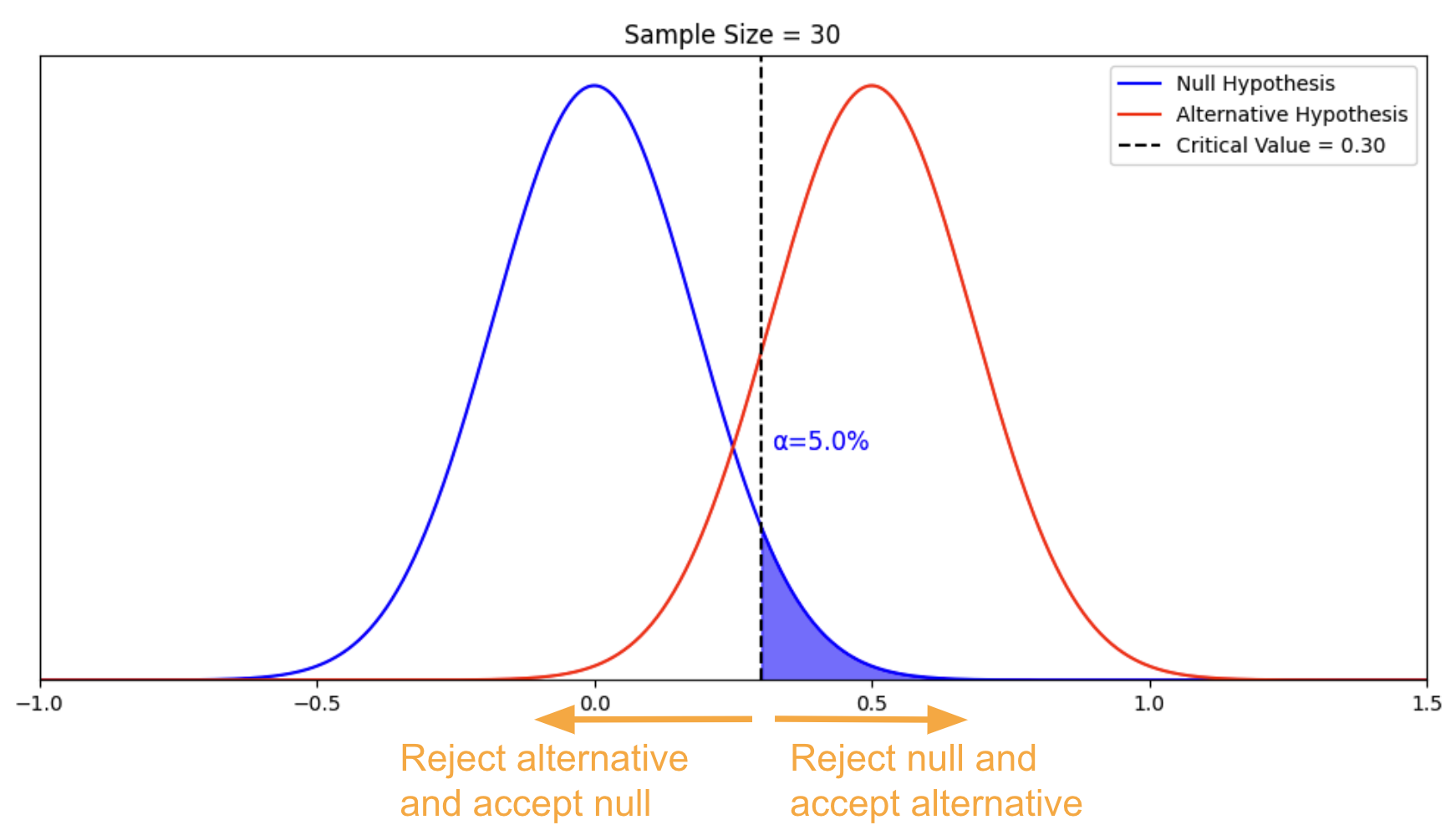
With the introduction of the alternative hypothesis, the alternative “(hypothesized) truth”, we can call “accepting the null hypothesis and rejecting the alternative hypothesis” a mistake – the Type II error. We can also calculate the probability of this mistake. This is called beta, which is illustrated by the red area below.

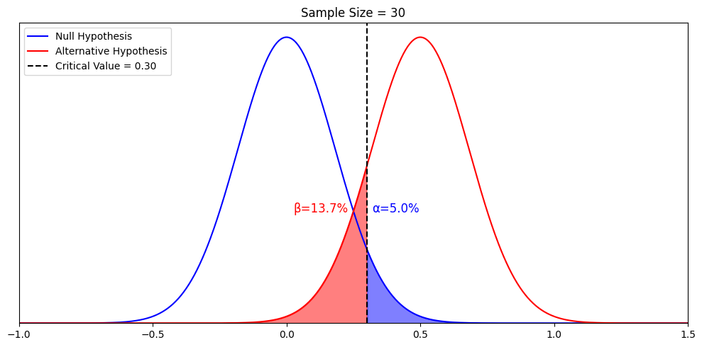
From the visualization, we can see that beta is conditional on the alternative hypothesis and the critical value. Let’s elaborate on these two relationships one by one, very explicitly, as both of them are important.

First, Let’s visualize how beta changes with the mean of the alternative hypothesis by setting another alternative hypothesis where mean = 1 instead of 0.5

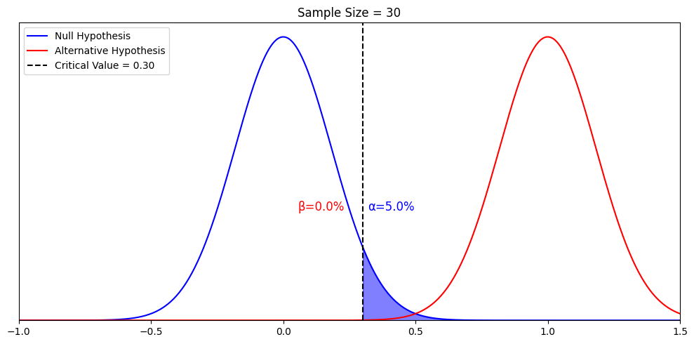
Beta change from 13.7% to 0.0%. Namely, beta is the probability of falsely rejecting a particular alternative hypothesis when we assume it is true. When we assume a different alternative hypothesis is true, we get a different beta. So strictly speaking, beta only speaks to the probability of falsely rejecting a particular alternative hypothesis when it is true . Nothing else. It’s only under other conditions, that “rejecting the alternative hypothesis” implies “accepting” the null hypothesis or “failing to accept the null hypothesis”. We will further elaborate when we talk about p-value and confidence interval in another article. But what we talked about so far is true and enough for understanding power.

Second, there is a relationship between alpha and beta. Namely, given the null hypothesis and the alternative hypothesis, alpha would determine the critical value, and the critical value determines beta. This speaks to the tradeoff between mistake and discovery. 

If we tolerate more alpha, we will have a smaller critical value, and for the same beta, we can detect a smaller alternative hypothesis

If we tolerate more beta, we can also detect a smaller alternative hypothesis. 

In short, if we tolerate more mistakes (either Type I or Type II), we can detect a smaller true effect. Mistake vs. discovery is the fundamental tradeoff of Hypothesis Testing.

So tolerating more mistakes leads to more chance of discovery. This is the concept of MDE that we will elaborate on in part 4.

Finally, we’re ready to define power. Power is an important and fundamental topic in statistical testing, and we’ll explain the concept in three different ways.

Three ways to understand power

First, the technical definition of power is 1−β. It represents that given an alternative hypothesis and given our null, sample size, and decision rule (alpha = 0.05), the probability is that we accept this particular hypothesis. We visualize the yellow area below.

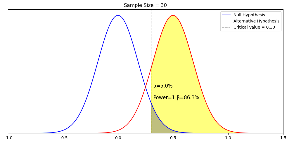
Second, power is really intuitive in its definition. A real-world example is trying to determine the most popular car manufacturer in the world. If I observe one car and see one brand, my observation is not very powerful. But if I observe a million cars, my observation is very powerful. Powerful tests mean that I have a high chance of detecting a true effect.

Third, to illustrate the two concepts concisely, let’s run a visualization by just changing the sample size from 30 to 100 and see how power increases from 86.3% to almost 100%.

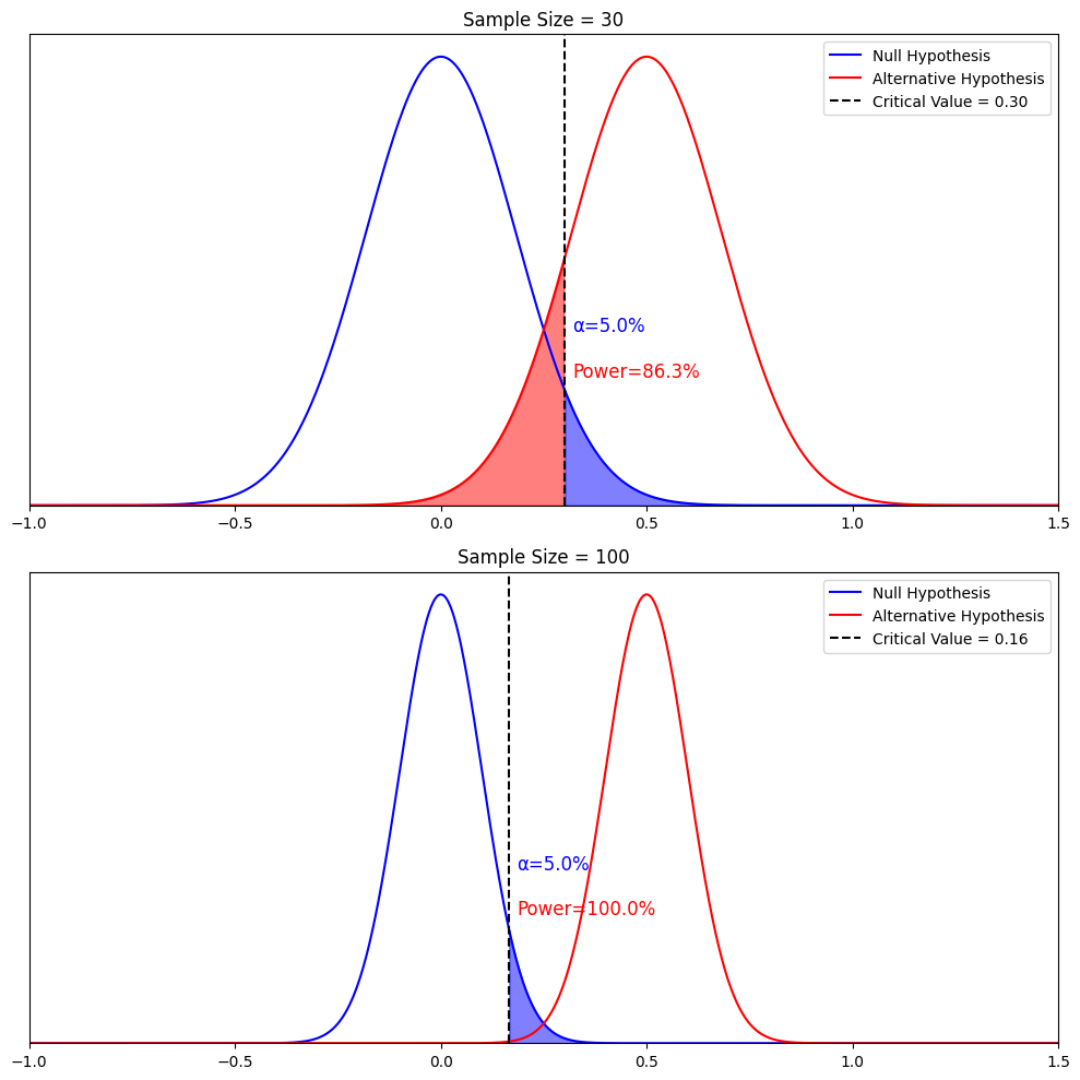
As the graph shows, we can easily see that power increases with sample size . The reason is that the distribution of both the null hypothesis and the alternative hypothesis became narrower as their sample means got more accurate. We are less likely to make either a type I error (which reduces the critical value) or a type II error.  

Type II error: Failing to reject the null hypothesis when the alternative hypothesis is true

Beta: The probability of making a type II error

Power: The ability of the test to detect a true effect when it’s there

Part 4, Power calculation: MDE

The relationship between mde, alternative hypothesis, and power.

Now, we are ready to tackle the most nuanced definition of them all: Minimum detectable effect (MDE). First, let’s make the sample mean of the alternative hypothesis explicit on the graph with a red dotted line.

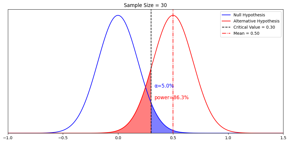
What if we keep the same sample size, but want power to be 80%? This is when we recall the previous chapter that “alternative hypotheses are theoretical constructs”. We can have a different alternative that corresponds to 80% power. After some calculations, we discovered that when it’s the alternative hypothesis with mean = 0.45 (if we keep the standard deviation to be 1).

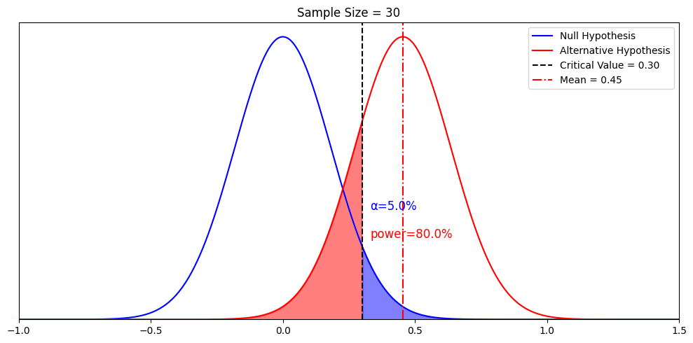
This is where we reconcile the concept of “infinitely many alternative hypotheses” with the concept of minimum detectable delta. Remember that in statistical testing, we want more power. The “ minimum ” in the “ minimum detectable effect”, is the minimum value of the mean of the alternative hypothesis that would give us 80% power. Any alternative hypothesis with a mean to the right of MDE gives us sufficient power.

In other words, there are indeed infinitely many alternative hypotheses to the right of this mean 0.45. The particular alternative hypothesis with a mean of 0.45 gives us the minimum value where power is sufficient. We call it the minimum detectable effect, or MDE.

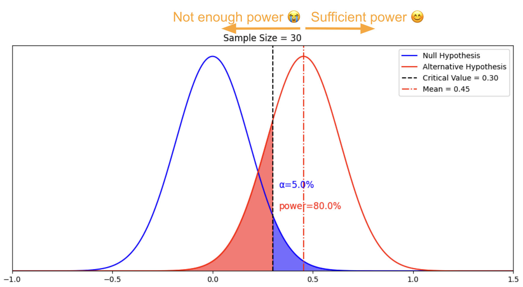
The complete definition of MDE from scratch

Let’s go through how we derived MDE from the beginning:

We fixed the distribution of sample means of the null hypothesis, and fixed sample size, so we can draw the blue distribution

For our decision rule, we require alpha to be 5%. We derived that the critical value shall be 0.30 to make 5% alpha happen

We fixed the alternative hypothesis to be normally distributed with a standard deviation of 1 so the standard error is 0.18, the mean can be anywhere as there are infinitely many alternative hypotheses

For our decision rule, we require beta to be 20% or less, so our power is 80% or more. 

We derived that the minimum value of the observed mean of the alternative hypothesis that we can detect with our decision rule is 0.45. Any value above 0.45 would give us sufficient power.

How MDE changes with sample size

Now, let’s tie everything together by increasing the sample size, holding alpha and beta constant, and see how MDE changes.

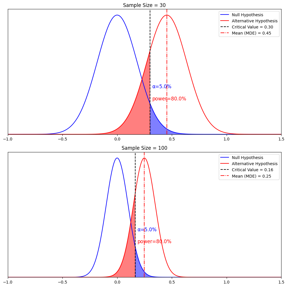
Narrower distribution of the sample mean + holding alpha constant -> smaller critical value from 0.3 to 0.16

+ holding beta constant -> MDE decreases from 0.45 to 0.25

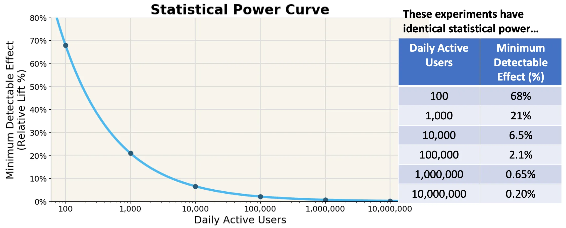
This is the other key takeaway:  The larger the sample size, the smaller of an effect we can detect, and the smaller the MDE.

This is a critical takeaway for statistical testing. It suggests that even for companies not with large sample sizes if their treatment effects are large, AB testing can reliably detect it.

Summary of Hypothesis Testing

Let’s review all the concepts together.

Assuming the null hypothesis is correct:

Alpha: When the null hypothesis is true, the probability of rejecting it

Critical value: The threshold to determine rejecting vs. accepting the null hypothesis

Assuming an alternative hypothesis is correct:

Beta: When the alternative hypothesis is true, the probability of rejecting it

Power: The chance that a real effect will produce significant results

Power calculation:

Minimum detectable effect (MDE): Given sample sizes and distributions, the minimum mean of alternative distribution that would give us the desired alpha and sufficient power (usually alpha = 0.05 and power >= 0.8)

Relationship among the factors, all else equal: Larger sample, more power; Larger sample, smaller MDE

Everything we talk about is under the Neyman-Pearson framework. There is no need to mention the p-value and significance under this framework. Blending the two frameworks is the inconsistency brought by our textbooks. Clarifying the inconsistency and correctly blending them are topics for another day.

Practical recommendations

That’s it. But it’s only the beginning. In practice, there are many crafts in using power well, for example:

Why peeking introduces a behavior bias, and how to use sequential testing to correct it

Why having multiple comparisons affects alpha, and how to use Bonferroni correction

The relationship between sample size, duration of the experiment, and allocation of the experiment?

Treat your allocation as a resource for experimentation, understand when interaction effects are okay, and when they are not okay, and how to use layers to manage

Practical considerations for setting an MDE

Also, in the above examples, we fixed the distribution, but in reality, the variance of the distribution plays an important role. There are different ways of calculating the variance and different ways to reduce variance, such as CUPED, or stratified sampling.

Related resources:

How to calculate power with an uneven split of sample size: https://blog.statsig.com/calculating-sample-sizes-for-a-b-tests-7854d56c2646

Real-life applications: https://blog.statsig.com/you-dont-need-large-sample-sizes-to-run-a-b-tests-6044823e9992

Create a free account

2m events per month, free forever..

Sign up for Statsig and launch your first experiment in minutes.

Build fast?

Try statsig today.

Recent Posts

Building an experimentation platform: assignment.

Take an inside look at how we built Statsig, and why we handle assignment the way we do.   Read More ⇾

Decoding metrics and experimentation with Ron Kohavi

Learn the takeaways from Ron Kohavi's presentation at Significance Summit wherein he discussed the challenges of experimentation and how to overcome them.   Read More ⇾

It’s normal not to be normal(ly distributed): what to do when data is not normally distributed

Learn how the iconic t-test adapts to real-world A/B testing challenges and discover when alternatives might deliver better results for your experiments.   Read More ⇾

How the engineers building Statsig solve hundreds of customer problems a week

See how we’re making support faster, smarter, and more personal for every user by automating what we can, and leveraging real, human help from our engineers.   Read More ⇾

Enhanced marketing experiments with Statsig Warehouse Native

Marketing platforms offer basic A/B testing, but their analysis tools fall short. Here's how Statsig helps you bridge the gap and unlock deeper insights.   Read More ⇾

Feature rollouts: How Instagram left me behind

When Instagram Stories rolled out, many of us were left behind, giving us a glimpse into the secrets behind Meta’s rollout strategy and tech’s feature experiments.   Read More ⇾